
Spatiotemporal coordinated air-to-ground attack strategy of an unmanned aerial vehicle swarm
-
摘要:
针对三维战场环境下无人机集群协同对地打击问题,提出了一种基于预设时间收敛的无人机集群时空协同控制方法. 首先,对无人机集群对地攻击任务场景及其相关要素进行了分析,并建立了无人机集群、地面运动目标和攻击问题模型. 在问题建模的基础上,考虑无人机集群的时空协同策略,设计三维空间无人机集群对地攻击的时空协同控制律. 所提出的时空协同控制律能够控制无人机集群在指定的时间内到达期望的攻击位置,实现对地面运动目标的时空协同攻击. 通过基于李雅普诺夫函数的理论分析,证明了所提出的控制律能够在预设时间条件下使攻击位置误差变量渐进稳定. 仿真结果表明,在地面运动目标转弯运动的情况下,所提出的协同控制律能够实现无人机集群的时空协同,在指定的时间内完成对地面运动目标的多角度协同攻击.
Abstract:This paper proposes a spatiotemporal coordinated control method for unmanned aerial vehicle (UAV) swarms based on predefined time convergence in response to the coordinated ground attack problem of UAV swarms in a three-dimensional battlefield environment. First, we analyze the UAV swarm’s ground attack task scenario and its relevant elements and establish models for the UAV swarm, ground-moving targets, and attack problems. Building upon problem modeling, this paper considers the spatiotemporal coordinated strategy for a UAV swarm and designs a spatiotemporal coordinated control law for a three-dimensional spatial UAV swarm ground attack. The proposed spatiotemporal coordinated control law can guide the UAV swarm to reach the desired attack position within a specified time, achieving a spatiotemporal coordinated attack on ground-moving targets. A theoretical analysis based on the Lyapunov function demonstrates that the proposed control law can asymptotically stabilize the attack position error variable under a predefined time condition. Simulation results show that the proposed coordinated control law can achieve spatiotemporal coordination of the UAV swarm in a ground-moving target turning motion, enabling the completion of the multiangle coordinated attack on ground-moving targets within a specified time. Currently, research on the coordinated ground attack of UAV swarms mostly focuses on stationary targets, making it difficult to apply to coordinated attack tasks on moving targets. Although the coordinated tracking of moving targets by UAV swarms has been reported in the literature, spatiotemporal coordination among UAVs has not been considered. Therefore, this paper focuses on the spatiotemporal coordinated control strategy of UAV swarms, with a background of coordinated ground attacks by UAV swarms. First, this paper conducts a detailed analysis of the UAV swarm’s coordinated ground attack task in terms of time and multiple elements to establish a comprehensive task profile. Subsequently, by focusing on the core elements of coordinated ground attack by UAV swarms, this paper models both UAV swarms and ground-moving targets. Based on the established models and coordinated control strategy, this paper considers spatiotemporal coordination constraints and designs acceleration commands for each UAV to guide them to reach the specified attack positions at predefined time points, enabling coordinated attacks on the ground targets simultaneously. The designed acceleration control commands serve as inputs to the UAV’s autopilot, further generating lower-level control commands, such as speed, flight path angle, and heading angle, thereby achieving stable flight control of the UAVs. The proposed coordinated control strategy endows the UAV swarm with the capability to achieve spatiotemporal synchronized coordinated attacks, thereby enhancing the operational effectiveness of UAV-coordinated ground attacks.
-
Keywords:
- UAV swarm /
- ground attack /
- spatiotemporal coordination /
- ground-moving targets /
- predetermined time
-
公开报道的无人机集群作战的首个战例发生于2018年1月,叙利亚反对派出动13架小型攻击无人机,对俄罗斯的赫梅米姆空军基地和塔尔图斯港补给站展开集群式攻击. 面向现代局部战争的新要求,无人机集群作战打破传统单机执行任务的局限,利用数架无人机对地面目标协同打击,能够有效提升突防概率和毁伤效能,将成为未来战争中一种重要的作战样式[1−5]. 因此,研究无人机集群协同对地攻击具有重要实际意义.
针对无人机集群协同对地攻击任务,通过美海军对无人机集群攻击情况的研究发现,时间和空间协同策略可以提升饱和攻击能力,最大程度发挥无人机集群整体效能. 时间协同主要包括同时到达、时序到达和定时到达,空间协同主要包括攻击位置协同和攻击进入角度协同[6−12]. 针对无人机集群协同对地攻击问题,目前实现无人机时空协同控制的方法主要可分为两种:一是调整路径的方法,即保持无人机飞行速度为定值,仅调整每架无人机的航路长度. 文献[13]提出基于带有回旋弧的Dubins路径为每架无人机生成飞行路径,在满足安全飞行约束的基础上,协调每个飞行路径的长度,使所有路径的长度相等从而实现同时到达. 文献[14]采用PH(Pythagorean hodograph)路径进行攻击路径规划,该路径长度可通过调节参数来变化. 为了使每架无人机路径长度相等,在适应度函数中考虑路径长度相等的因素,通过协同粒子群优化算法求解得到相同长度的攻击路径. 文献[15−16]同样采用Dubins路径来规划各无人机攻击路径,构建无人机攻击编组并提出协同战术,实现了无人机集群以特定的攻击角度对地面静止目标协同攻击. 二是调整速度的方法,即在规划好每架无人机攻击路径的基础上,通过调整无人机的速度来实现时间协同. 文献[17]提出了基于一致性的无人机协同控制算法,该方法假定无人机飞行路径已知,通过不断调整每架无人机的速度,实现各无人机到达时间的渐进一致,最终完成无人机集群同时到达任务点. 在文献[17]研究基础上,文献[18]引入外部参考信号,考虑虚拟领导者的编队结构,提出了基于一致性算法的协同控制方法,该方法可以实现在路径误差和突发威胁等不利因素的条件下,无人机集群仍能同时到达任务点. 此外,综合上述两种方法的优势,文献[19]考虑突发威胁的情况,在攻击过程中重新规划攻击路径并实时调整速度,具有更好的动态适应性.
目前,无人集群协同对地攻击问题的研究大多针对静止目标展开,难以适用于运动目标的协同攻击任务[20]. 即使部分文献对无人机集群协同跟踪运动目标问题开展研究,但未考虑到各无人机间时空协同的因素[21]. 因此,本文以无人机集群协同对地面运动目标攻击为背景,重点研究无人机集群时空协同控制策略. 首先,对无人机集群协同对地攻击任务进行分时序、多要素剖析,建立完整的任务剖面. 其次,针对无人机集群协同对地攻击问题中的核心要素,对无人机集群和地面运动目标进行建模. 在模型建立的基础上,基于协同控制策略,考虑时空协同约束条件,通过设计每架无人机的加速度指令,引导各无人机在预设时间点到达指定攻击阵位,完成同一时间对地面目标的协同打击. 设计的加速度控制指令作为无人机自动驾驶仪的输入,进一步生成飞机的速度、航迹角、航向角等底层控制指令,实现无人机的稳定飞行控制. 本文提出的无人机集群协同控制策略,赋予了无人机集群时空同步协同打击能力,提升了无人机协同对地攻击的作战效能.
1. 无人机集群对地攻击时空协同问题建模
1.1 问题描述
由n架攻击型无人机组成的无人机集群,执行时空协同对地攻击任务,场景示意图如图1所示. 通过对分布在不同位置的多架攻击型无人机进行时空协同控制,使其在特定时间从多个攻击角度同时到达地面移动目标的相对预设攻击阵位,要求不仅无人机与目标之间相对位置关系要满足攻击要求,而且相对速度和进入攻击角度也应该保持在特定的范围内.
![]() 图 1 无人机集群时空协同对地攻击任务示意图Figure 1. UAV formation spatiotemporal coordinated ground attack task
图 1 无人机集群时空协同对地攻击任务示意图Figure 1. UAV formation spatiotemporal coordinated ground attack task具体地,考虑三维空间中无人机集群对运动目标实施时空协同攻击. 图2给出了无人机集群中第$ i $架无人机与运动目标相对位置和速度关系,其中I点、T点和D点分别表示无人机、运动目标和期望攻击阵位点. 基于惯性坐标系,第$ i $架无人机的位置、速度和加速度分别表示为$ {{\boldsymbol{r}}_i} = {[{x_i},{y_i},{z_i}]^{\text{T}}} $,$ {{\boldsymbol{v}}_i} = {[{v_{ix}},{v_{iy}},{v_{iz}}]^{\text{T}}} $和$ {{\boldsymbol{a}}_i} = {[{a_{ix}},{a_{iy}},{a_{iz}}]^{\text{T}}} $;运动目标的位置、速度和加速度分别表示为$ {{\boldsymbol{r}}_t} = {[{x_t},{y_t},{z_t}]^{\text{T}}} $,$ {{\boldsymbol{v}}_t} = {[{v_{tx}},{v_{ty}},{v_{tz}}]^{\text{T}}} $和$ {{\boldsymbol{a}}_t} = {[{a_{tx}},{a_{ty}},{a_{tz}}]^{\text{T}}} $;对应第$ i $架无人机的期望攻击阵位点的位置、速度和加速度可分别表示为$ {{\boldsymbol{r}}_{{\mathrm{d}}i}} = {[{x_{{\mathrm{d}}i}},{y_{{\mathrm{d}}i}},{z_{{\mathrm{d}}i}}]^{\text{T}}} $,$ {{\boldsymbol{v}}_{{\mathrm{d}}i}} = {[{v_{{\mathrm{d}}ix}},{v_{{\mathrm{d}}iy}},{v_{{\mathrm{d}}iz}}]^{\text{T}}} $和$ {{\boldsymbol{a}}_{{\mathrm{d}}i}} = [{a_{{\mathrm{d}}ix}}, {a_{{\mathrm{d}}iy}}, {a_{{\mathrm{d}}iz}}]^{\text{T}} $. 因此,第$ i $架无人机与其期望攻击阵位点之间的相对位置、速度以及加速度可分别表示为$ \Delta {{\boldsymbol{r}}_{{\mathrm{d}}i}} = {{\boldsymbol{r}}_{{\mathrm{d}}i}} - {{\boldsymbol{r}}_i} $,$ \Delta {{\boldsymbol{v}}_{{\mathrm{d}}i}} = {{\boldsymbol{v}}_{{\mathrm{d}}i}} - {{\boldsymbol{v}}_i} $和$ \Delta {{\boldsymbol{a}}_{{\mathrm{d}}i}} = {{\boldsymbol{a}}_{{\mathrm{d}}i}} - {{\boldsymbol{a}}_i} $.
![]() 图 2 无人机与运动目标相对位置和速度关系示意图Figure 2. Relative position and velocity relationship between the UAV and the target
图 2 无人机与运动目标相对位置和速度关系示意图Figure 2. Relative position and velocity relationship between the UAV and the target1.2 无人机运动模型
为更清楚地描述无人机集群与地面移动目标间的相对位置、速度、航向角的变化规律,需建立无人机运动模型(图3). 为简化模型的建立,给出如下合理的假设:1)无人机均装备有定位系统和地面移动目标指示雷达,能够确定地面移动目标的位置和速度信息;2)无人机飞行过程中不会收到外界大幅扰动影响,飞行状态平稳;3)无人机自身装有飞行控制系统,其底层控制指令可由系统自动解算. 基于上述假设成立,建立下列三自由度无人机运动学模型:
$$ \left\{ \begin{gathered} {{\dot x}_i}(t) = {V_i}(t)\cos {\gamma _i}(t)cos{\psi _i}(t) \\ {{\dot y}_i}(t) = {V_i}(t)\cos {\gamma _i}(t)\sin {\psi _i}(t) \\ {{\dot z}_i}(t) = {V_i}(t)\sin {\gamma _i}(t) \\ {{\dot V}_i}(t) = \frac{{{T_{{\text{h}}i}}(t) - {D_{{\text{g}}i}}(t)}}{{{m_i}}} - {g_{\text{a}}}\sin {\gamma _i}(t) \\ {{\dot \gamma }_i}(t) = \frac{{{g_{\text{a}}}}}{{{V_i}(t)}}\left( {{n_{{\text{g}}i}}(t)\cos {\phi _i}(t) - \cos {\gamma _i}(t)} \right) \\ {{\dot \psi }_i}(t) = \frac{{{L_{{\text{f}}i}}(t)\sin {\phi _i}(t)}}{{{m_i}{V_i}(t)\cos {\gamma _i}(t)}} \\ \end{gathered} \right. $$ (1) 其中,$ i = 1, \cdots ,n $表示无人机的编号,$ n $为无人机数量,$ {x_i} $,$ {y_i} $分别表示无人机在惯性坐标系中的东向和北向坐标,$ {z_i} $表示飞行高度,$ {m_i} $为质量,$ {g_{\mathrm{a}}} $为重力加速度,$ {D_{{\mathrm{g}}i}} $为阻力,$ {L_{{\mathrm{f}}i}} $为升力,$ {V_i} $为地速,$ {\gamma _i} $为爬升角,$ {\psi _i} $为偏航角,$ {\phi _i} $为滚转角,$ {T_{{\mathrm{h}}i}} $表示发动机推力,$ {n_{{\mathrm{g}}i}} = {L_{{\mathrm{f}}i}}/({g_{\mathrm{a}}}{m_i}) $表示过载.
为便于问题求解,本文通过反馈线性化方法,将上述复杂的非线性无人机模型转化为线性二阶积分器模型[22−24],得到式(3)所示的线性模型:
$$ \left\{ \begin{gathered} {{\dot x}_i}(t) = {v_{xi}}(t);\quad {{\dot v}_{xi}}(t) = {a_{xi}}(t) \\ {{\dot y}_i}(t) = {v_{yi}}(t);\quad {{\dot v}_{yi}}(t) = {a_{yi}}(t) \\ {{\dot z}_i}(t) = {v_{zi}}(t);\quad {{\dot v}_{zi}}(t) = {a_{zi}}(t) \\ \end{gathered} \right. $$ (2) 其中,$ {a_{xi}} $,$ {a_{yi}} $,$ {a_{zi}} $为二阶积分器模型中的控制输入,该控制输入与无人机实际控制量之间存在下列关系:
$$ \begin{split} &{\phi _i} = {\tan ^{ - 1}}\left[ {\frac{{{a_{yi}}\cos {\psi _i} - {a_{xi}}\sin{\psi _i}}}{{\cos {\gamma _i}({a_{zi}} + {g_{\mathrm{a}}}) - \sin {\gamma _i}({a_{xi}}\cos {\psi _i} + {a_{yi}}\sin{\psi _i})}}} \right] \\ &{n_{{\mathrm{g}}i}} = \frac{{\cos {\gamma _i}({a_{zi}} + {g_{\mathrm{a}}}) - \sin {\gamma _i}({a_{xi}}\cos {\psi _i} + {a_{yi}}\sin{\psi _i})}}{{{g_{\mathrm{a}}}\cos {\phi _i}}} \\ & {T_{{\mathrm{h}}i}} = \left[ {\sin {\gamma _i}({a_{zi}} + {g_{\mathrm{a}}}) + \cos {\gamma _i}({a_{xi}}\cos {\psi _i} + {a_{yi}}\sin{\psi _i})} \right]{m_i} +\\ &\qquad\;\;{D_{{\mathrm{g}}i}}\\[-1pt] \end{split} $$ (3) 通过设计控制律$ {{\boldsymbol{a}}_{{\mathrm{u}}i}} = {[ {{a_{xi}},{a_{yi}},{a_{zi}}} ]^T} $,并根据式(3)可求解得到实际控制量$ {n_{{\mathrm{g}}i}} $,$ {\phi _i} $和$ {T_{{\mathrm{h}}i}} $. 无人机机载计算机解算出实际控制量后发送给飞行控制系统,飞行控制系统能够自主计算出升降舵、方向舵、副翼的舵偏角和油门大小,进而控制无人机的飞行.
1.3 目标运动模型
目标是指无人机集群攻击的对象. 按照运动特性划分,可以将目标分为静止目标和运动目标. 本文主要针对无人机集群对地面运动目标协同攻击问题展开研究,定义地面运动目标状态为$ {{\boldsymbol{X}}_{\mathrm{r}}}\left( t \right) = $ $ {[{x_{\mathrm{r}}}(t),{y_{\mathrm{r}}}(t),{z_{\mathrm{r}}}(t),{v_{x{\mathrm{r}}}}(t),{v_{y{\mathrm{r}}}}(t),{v_{z{\mathrm{r}}}}(t)]^{\text{T}}} $,其中$ {x_{\mathrm{r}}}(t) $,$ {y_{\mathrm{r}}}(t) $,$ {z_{\mathrm{r}}}(t) $表示目标的三维位置坐标,$ {v_{x{\mathrm{r}}}}(t) $,$ {v_{y{\mathrm{r}}}}(t) $,$ {v_{z{\mathrm{r}}}}(t) $分别表示运动目标速度在$ X $轴,$ Y $轴,$ Z $轴上速度分量. 目标的运动学模型可用下列方程表示:
$$ {\dot {\boldsymbol{X}}_{\mathrm{r}}}\left( t \right) = {{\boldsymbol{f}}_{\mathrm{r}}}\left( {{{\boldsymbol{X}}_{\mathrm{r}}},t} \right) + {{\boldsymbol{G}}_{\mathrm{r}}}{{\boldsymbol{U}}_{\mathrm{r}}} $$ (4) 其中,$ {{\boldsymbol{f}}_{\mathrm{r}}}\left( {{{\boldsymbol{X}}_{\mathrm{r}}},t} \right) $表示运动目标的非线性项,$ {{\boldsymbol{G}}_{\mathrm{r}}} $,$ {{\boldsymbol{U}}_{\mathrm{r}}} $分别表示运动目标控制增益和控制量.
2. 无人机集群对地攻击时空协同控制设计
2.1 控制器设计
根据问题描述,本节设计无人机集群协同控制器,实现预设时间条件下无人机集群时空协同对地攻击. 根据第$ i $架无人机与其期望攻击阵位点之间的相对位置$ \Delta {{\boldsymbol{r}}_{{\mathrm{d}}i}} $、速度$ \Delta {{\boldsymbol{v}}_{{\mathrm{d}}i}} $以及加速度$ \Delta {{\boldsymbol{a}}_{{\mathrm{d}}i}} $,定义如下攻击位置误差变量$ {{\boldsymbol{\varepsilon}} _i} $:
$$ {{\boldsymbol{\varepsilon }}_i} = \Delta {{\boldsymbol{r}}_{{\mathrm{d}}i}} + \Delta {{\boldsymbol{v}}_{{\mathrm{d}}i}}{t_{{\mathrm{go}}}} + \frac{1}{2}\Delta {{\boldsymbol{a}}_{{\mathrm{d}}i}}t_{{\mathrm{go}}}^2 $$ (5) 其中,$ {t_{{\mathrm{go}}}} = {t_{\mathrm{f}}} - t $,$ {t_{\mathrm{f}}} $表示预设攻击时间.
根据攻击位置误差变量$ {{\boldsymbol{\varepsilon}} _i} $,现给出下列李雅普诺夫函数:
$$ {L_i} = \frac{1}{2}\frac{{{\boldsymbol{\varepsilon}} _i^{\text{T}}{{\boldsymbol{\varepsilon}} _i}}}{{t_{{\mathrm{go}}}^2}} $$ (6) 求导上述李雅普诺夫函数$ {L_i} $得:
$$ {\dot L_i} = \frac{{{\boldsymbol{\varepsilon}} _i^{\text{T}}}}{{t_{{\mathrm{go}}}^3}}\left( {{{\boldsymbol{\varepsilon}} _i} + {{\dot {\boldsymbol{\varepsilon}} }_i}{t_{{\mathrm{go}}}}} \right) $$ (7) 将式(5)代入式(7)得:
$$ {\dot L_i} = \frac{{{\boldsymbol{\varepsilon}} _i^{\text{T}}}}{{t_{{\mathrm{go}}}^3}}\left( {{{\boldsymbol{\varepsilon}} _i} + \frac{1}{2}\Delta {{\dot {\boldsymbol{a}}}_{{\mathrm{d}}i}}t_{{\mathrm{go}}}^3} \right) $$ (8) 设计如下加速度控制律:
$$ \Delta {\dot {\boldsymbol{a}}_{{\text{d}}i}} = - \frac{{2{{\boldsymbol{\varepsilon}} _i}}}{{t_{{\mathrm{go}}}^3}} - {k_i}\frac{{2{{\boldsymbol{\varepsilon}} _i}}}{{t_{{\mathrm{go}}}^2}} $$ (9) 其中,控制参数$ {k_i} > 0 $.
$$ {\dot {\boldsymbol{a}}_i} = \frac{1}{{{\tau _{{\text{a}}i}}}}\left( {{\boldsymbol{a}}_i^{\mathrm{c}} - {{\boldsymbol{a}}_i}} \right) $$ (10) 其中,$ {\tau _{{\text{a}}i}} $为时间常数,$ {\boldsymbol{a}}_i^{\mathrm{c}} $表示加速度控制指令,$ {{\boldsymbol{a}}_i} $表示加速度.
根据$ \Delta {{\boldsymbol{a}}_{{\mathrm{d}}i}} = {{\boldsymbol{a}}_{{\mathrm{d}}i}} - {{\boldsymbol{a}}_i} $,代入式(10)可得:
$$ \Delta {\dot {\boldsymbol{a}}_{{\mathrm{d}}i}} = {\dot {\boldsymbol{a}}_{{\mathrm{d}}i}} - \frac{1}{{{\tau _{{\text{a}}i}}}}\left( {{\boldsymbol{a}}_i^{\mathrm{c}} - {{\boldsymbol{a}}_i}} \right) $$ (11) 根据式(9)可计算得到加速度控制指令$ {\boldsymbol{a}}_i^{\mathrm{c}} $
$$ {\boldsymbol{a}}_i^{\mathrm{c}} = {{\boldsymbol{a}}_i} + {\tau _{{\text{a}}i}}{\dot {\boldsymbol{a}}_{{\mathrm{d}}i}} + {\tau _{{\text{a}}i}}\frac{{\left( {{k_i}{t_{{\mathrm{go}}}} + 1} \right)}}{{t_{{\mathrm{go}}}^2}}{{\boldsymbol{\varepsilon}} _i} $$ (12) 通常大多数文献假设时间常数$ {\tau _{{\text{a}}i}} $为定常值,但在实际无人机系统中,$ {\tau _{{\text{a}}i}} $会随着加速度变化而改变,存在参数不确定性. 因此,定义$ {\tau _{{\text{a}}i}} = {\bar \tau _{{\text{a}}i}} + \Delta {\tau _{{\text{a}}i}} $,其中$ \Delta {\tau _{{\text{a}}i}} $表示$ {\tau _{{\text{a}}i}} $对应的不确定项,$ {\bar \tau _{{\text{a}}i}} $表示已知的基准时间常数. 基于$ {\bar \tau _{{\text{a}}i}} $,实际的加速度控制指令$ {\boldsymbol{a}}_i^{\mathrm{c}} $表示为
$$ {\boldsymbol{a}}_i^{\mathrm{c}} = {{\boldsymbol{a}}_i} + {\bar \tau _{{\text{a}}i}}{\dot {\boldsymbol{a}}_{{\mathrm{d}}i}} + {\bar \tau _{{\text{a}}i}}\frac{{\left( {{k_i}{t_{{\mathrm{go}}}} + 1} \right)}}{{t_{{\mathrm{go}}}^2}}{{\boldsymbol{\varepsilon}} _i} $$ (13) 2.2 稳定性证明
定理1:考虑一阶自动驾驶仪中时间常数$ {\tau _{{\text{a}}i}} $的不确定性,基于设计的加速度控制指令(13),可实现预设时间条件下攻击位置误差变量$ {{\boldsymbol{\varepsilon}} _i} $渐进稳定,即$ {{\boldsymbol{\varepsilon}} _i} $在预设时间点收敛到原点附近任意小的邻域内.
证明:根据设计的实际加速度控制指令$ {\boldsymbol{a}}_i^{\mathrm{c}} $,将式(13)代入式(11)得:
$$ \begin{split} \Delta {{\dot {\boldsymbol{a}}}_{{\mathrm{d}}i}} =\;& {{\dot {\boldsymbol{a}}}_{{\mathrm{d}}i}} - \frac{1}{{{\tau _{{\text{a}}i}}}}\left( {{{\boldsymbol{a}}_i} + {{\bar \tau }_{{\text{a}}i}}{{\dot {\boldsymbol{a}}}_{{\mathrm{d}}i}} + {{\bar \tau }_{{\text{a}}i}}\frac{{\left( {{k_i}{t_{{\mathrm{go}}}} + 1} \right)}}{{t_{{\mathrm{go}}}^2}}{{\boldsymbol{\varepsilon}} _i} - {{\boldsymbol{a}}_i}} \right) \\ =\;& {{\dot {\boldsymbol{a}}}_{{\mathrm{d}}i}} - \frac{{{{\bar \tau }_{{\text{a}}i}}}}{{{\tau _{{\text{a}}i}}}}\left( {{{\dot {\boldsymbol{a}}}_{{\mathrm{d}}i}} + \frac{{\left( {{k_i}{t_{{\mathrm{go}}}} + 1} \right)}}{{t_{{\mathrm{go}}}^2}}{{\boldsymbol{\varepsilon}} _i}} \right) \\ =\; & - \frac{{\Delta {\tau _{{\text{a}}i}}}}{{{\tau _{{\text{a}}i}}}}{{\dot {\boldsymbol{a}}}_{{\mathrm{d}}i}} - \frac{{{{\bar \tau }_{{\text{a}}i}}}}{{{\tau _{{\text{a}}i}}}}\frac{{\left( {{k_i}{t_{{\mathrm{go}}}} + 1} \right)}}{{t_{{\mathrm{go}}}^2}}{{\boldsymbol{\varepsilon}} _i} \\[-1pt] \end{split} $$ (14) 根据式(14),代入式(8)可知:
$$ \begin{split} {{\dot L}_i} = \;&\frac{{{\boldsymbol{\varepsilon}} _i^{\text{T}}}}{{t_{{\mathrm{go}}}^3}}\left( {{{\boldsymbol{\varepsilon}} _i} + \frac{1}{2}\Delta {{\dot {\boldsymbol{a}}}_{{\mathrm{d}}i}}t_{{\mathrm{go}}}^3} \right) \\ =\;& \frac{{{\boldsymbol{\varepsilon}} _i^{\text{T}}{{\boldsymbol{\varepsilon }}_i}}}{{t_{{\mathrm{go}}}^3}} - {\boldsymbol{\varepsilon}} _i^{\text{T}}\left( {\frac{{\Delta {\tau _{{\text{a}}i}}}}{{2{\tau _{{\text{a}}i}}}}{{\dot {\boldsymbol{a}}}_{{\mathrm{d}}i}} + \frac{{{{\bar \tau }_{{\text{a}}i}}}}{{{\tau _{{\text{a}}i}}}}\frac{{\left( {{k_i}{t_{{\mathrm{go}}}} + 1} \right)}}{{2t_{{\mathrm{go}}}^2}}{{\boldsymbol{\varepsilon}} _i}} \right) \\ =\;& - \frac{{\Delta {\tau _{{\text{a}}i}}}}{{2{\tau _{{\text{a}}i}}}}{\boldsymbol{\varepsilon }}_i^{\text{T}}{{\dot {\boldsymbol{a}}}_{{\mathrm{d}}i}} - \left( {\frac{{{{\bar \tau }_{{\text{a}}i}}}}{{{\tau _{{\text{a}}i}}}}\frac{{\left( {{k_i}{t_{{\mathrm{go}}}} + 1} \right)}}{{2t_{{\mathrm{go}}}^2}} - \frac{1}{{t_{{\mathrm{go}}}^3}}} \right){\boldsymbol{\varepsilon}} _i^{\text{T}}{{\boldsymbol{\varepsilon }}_i} \end{split} $$ (15) 在不考虑地面运动目标做不规则变加速的情况下,即$ {\dot {\boldsymbol{a}}_{{\mathrm{d}}i}} = {\boldsymbol{0}} $,化简式(15)可得:
$$ {\dot L_i} = - \left( {\frac{{{{\bar \tau }_{{\text{a}}i}}}}{{{\tau _{{\text{a}}i}}}}\frac{{\left( {{k_i}{t_{{\mathrm{go}}i}} + 1} \right)}}{{2t_{{\mathrm{go}}}^2}} - \frac{1}{{t_{{\mathrm{go}}}^3}}} \right){\boldsymbol{\varepsilon}} _i^{\text{T}}{{\boldsymbol{\varepsilon}} _i} $$ (16) 选取$ {k_i} $满足下列不等式成立:
$$ \frac{{{{\bar \tau }_{{\text{a}}i}}}}{{{\tau _{{\text{a}}i}}}}\frac{{\left( {{k_i}{t_{{\mathrm{go}}}} + 1} \right)}}{{2t_{{\mathrm{go}}}^2}} - \frac{1}{{t_{{\mathrm{go}}}^3}} > 0 $$ (17) 假设$ {\tau _{{\text{a}}i}} $存在参数不确定性,但满足在一定可控范围内变化,即$ {\tau _{\min }} \leqslant {\tau _{{\text{a}}i}} \leqslant {\tau _{\max }} $. 因此,化简式(17)可得:
$$ {k_i} > \frac{{2{\tau _{\max }}}}{{{{\bar \tau }_{{\text{a}}i}}t_{{\mathrm{go}}}^2}} - \frac{1}{{{t_{{\mathrm{go}}}}}} $$ (18) 当$ {k_i} $满足式(18)的不等式条件时,存在$ {\dot L_i} < 0 $,即证明预设时间条件下攻击位置误差变量$ {{\boldsymbol{\varepsilon }}_i} $渐进稳定收敛.
3. 仿真分析
3.1 有效性验证
本节对所提出时间协同控制律(13)的有效性进行验证. 首先对地面运动目标的运动进行描述,支撑后续控制律的验证. 假设地面目标为公路行驶的车辆,不考虑运动过程中的高度起伏,设定目标初始位置设为原点,目标的初始速度为$ {{\boldsymbol{v}}_t} = [15, 15,0]^{\text{T}} $. 攻击过程中,无人机编队只能获取到目标当前实时状态,目标未来的运动状态是未知的.
无人机编队的期望攻击阵位落在以地面目标为圆心,半径为1 m圆周等分的6个点上(如图4(b)所示),攻击高度为1 m,不同无人机从攻击圆上不同攻击角度进入打击,对应的攻击角度分别为0°,60°,120°,180°,240°,300°. 无人机的初始位置、初始速度、期望攻击阵位和期望到达时间如表1所示.
![]() 图 4 无人机编队对地攻击时空协同轨迹图. (a)三维轨迹图; (b)轨迹俯视图Figure 4. Spatiotemporal collaborative three-dimensional trajectory of a UAV swarm: (a) three-dimensional trajectory diagram; (b) top view of the track表 1 仿真参数设置Table 1. Simulation parameter settings
图 4 无人机编队对地攻击时空协同轨迹图. (a)三维轨迹图; (b)轨迹俯视图Figure 4. Spatiotemporal collaborative three-dimensional trajectory of a UAV swarm: (a) three-dimensional trajectory diagram; (b) top view of the track表 1 仿真参数设置Table 1. Simulation parameter settingsNumber Initial position/m Initial velocity/(m·s−1) Desired relative position/m Preset time/s 1 (−1200, 1300, 660) (40, 5, 0) (0.5, 0.87, 1) 100 2 (1300, 2300, 550) (30, −15, 0) (1, 0, 1) 100 3 (−1300, −800, 560) (25, −25, 0) (0.5, −0.87, 1) 100 4 (−1700, 500, 570) (15, −30, 0) (−0.5, −0.87, 1) 100 5 (−1100, −600, 640) (25, 25, 0) (−1, 0, 1) 100 6 (500, 2500, 660) (−25, −25, 0) (−0.5, 0.87, 1) 100 无人机编队对地攻击时空协同策略的仿真结果如图4所示. 图4(a)和图4(b)分别展示了协同攻击的三维轨迹及其俯视图,其中黑色虚线为地面车辆的运动轨迹. 由图4(b)可以看出6架无人机最终的攻击阵位落在以地面目标为圆心,半径为1 m圆周等分的6个点上,对应的攻击角度分别为0°,60°,120°,180°,240°,300°,形成了时空协同攻击的良好态势. 此种对地攻击策略意在实现无人机从不同角度协同打击,增强协同打击效果. 为更好地展示无人机编队对地攻击时空协同的动态过程,将仿真数据按照ACMI协议进行打包,导入TacView软件进行可视化显示. 图5给出了时间为0、50、80和100 s时TacView的可视化界面截图. 从图5中可以看出,初始阶段分散的无人机编队,通过本文设计的控制律(13),能够从不同方向同时对目标发起攻击. 图5(d)展示了最终完成时空协同的画面,表明所设计的控制律能够实现无人机编队时空协同对地攻击策略.
![]() 图 5 无人机编队对地攻击时空协同轨迹TacView可视化. (a) t=0 s; (b) t=50 s; (c) t=80 s; (d) t=100 sFigure 5. Spatiotemporal collaborative three-dimensional trajectory of UAV swarm rendered in TacView: (a) t=0 s; (b) t=50 s; (c) t=80 s; (d) t=100 s
图 5 无人机编队对地攻击时空协同轨迹TacView可视化. (a) t=0 s; (b) t=50 s; (c) t=80 s; (d) t=100 sFigure 5. Spatiotemporal collaborative three-dimensional trajectory of UAV swarm rendered in TacView: (a) t=0 s; (b) t=50 s; (c) t=80 s; (d) t=100 s在此基础上,计算得出:图6(a)所示的各无人机与目标相对速度曲线,相对速度有效控制在0~60 m·s−1范围内,符合无人机实际飞行能力;图6(b)所示的各无人机与地面目标的相对角度变化曲线,满足各无人机多轴向到达各自的期望攻击阵位的任务要求;以及图7所示的无人机过载变化曲线,各无人机过载的变化始终维持在[−0.4,0.3]之间,满足无人机动力学的约束条件.
![]() 图 6 无人机与目标相对速度及攻击角度. (a) 无人机与目标相对速度曲线; (b) 无人机进入攻击角度曲线Figure 6. Relative speed and attack angle of UAVs and target: (a) relative speed curve of UAVs and target; (b) attack angle curve of UAVs
图 6 无人机与目标相对速度及攻击角度. (a) 无人机与目标相对速度曲线; (b) 无人机进入攻击角度曲线Figure 6. Relative speed and attack angle of UAVs and target: (a) relative speed curve of UAVs and target; (b) attack angle curve of UAVs图8给出了各无人机速度和加速度的变化曲线. 如图8所示,各无人机速度变化平滑连续,符合实际情况. 从图8右图可以看出,由于目标在40~50 s时正在做转弯运动,造成无人机加速度在部分时间段内发生变化,但始终稳定在合理范围内,满足无人机控制约束条件要求.
图9给出了无人机与目标之间的水平相对距离随时间的变化曲线. 由图9可以看出,当t=100 s时,无人机编队中所有无人机与目标的相对距离同时接近于期望值. 从仿真结果来看,本文提出的协同攻击控制律能够较好的实现协同攻击过程中的时间和空间协同策略.
上述数值仿真表明所提出的协同攻击控制律能够控制无人机以指定的末端时间到达期望攻击阵位,完成时空协同攻击,验证了所提出控制律的有效性和理论分析的正确性.
3.2 对比验证
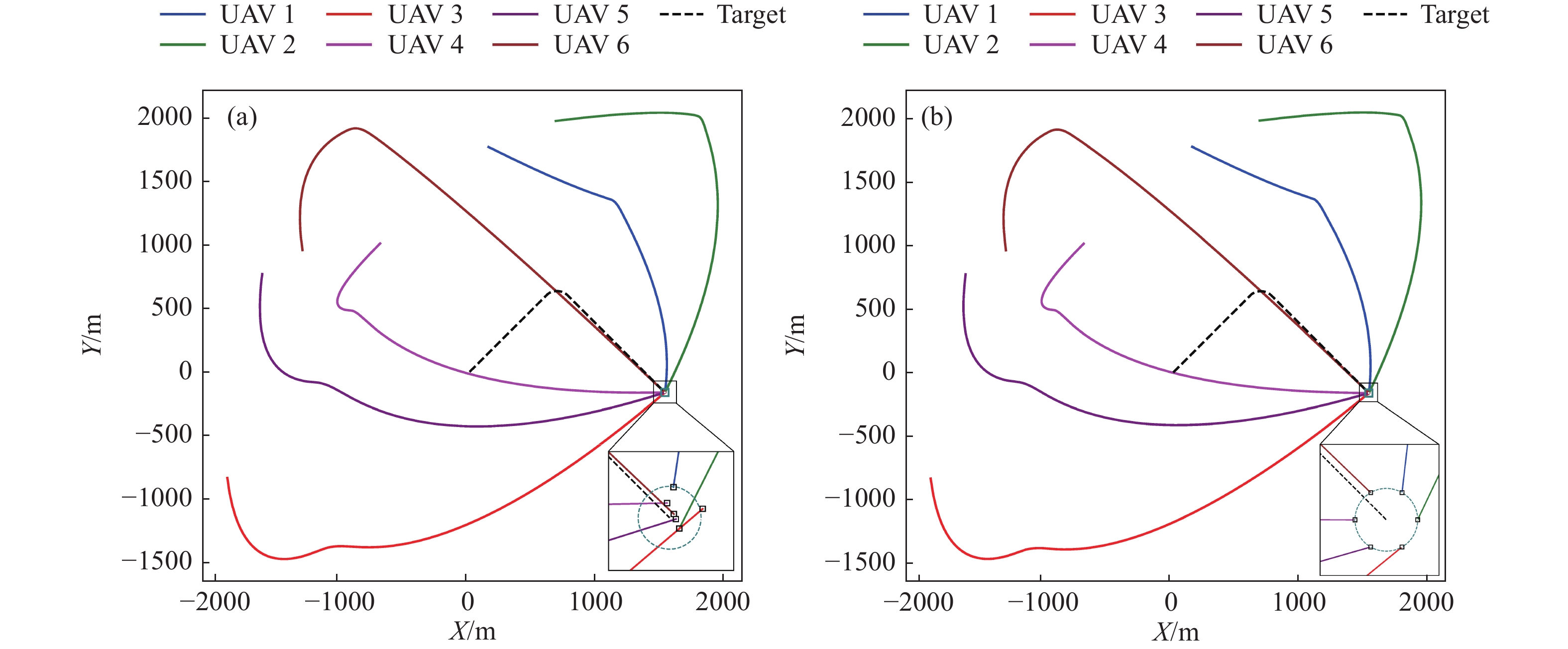
为更好地验证本文提出控制方法相较于经典PID算法的优越性,增设一组对比仿真实验. 选择不同于3.1节中仿真场景,改变各无人机的初始位置及初始速度,如表2所示. 无人机编队的期望攻击阵位同样落在以地面目标为圆心,半径为1 m圆周等分的6个点上(如图10(b)所示),攻击高度为1 m,不同无人机对应的攻击角度分别为0°,60°,120°,180°,240°,300°.
表 2 对比仿真参数设置Table 2. Simulation Parameter SettingsNumber Initial position/m Initial velocity/(m·s−1) Desired relative position/m Preset time/s 1 (149, 1771, 501) (30, −15, 0) (0.5, 0.87, 1) 100 2 (679, 1976, 520) (40, 5, 0) (1, 0, 1) 100 3 (−1906, −833, 547) (5, −40, 0) (0.5, −0.87, 1) 100 4 (−704, 1011, 595) (−25, −25, 0) (−0.5, −0.87, 1) 100 5 (−1632, 770, 657) (−5, −40, 0) (−1, 0, 1) 100 6 (−1315, 959, 618) (−5, 35, 0) (−0.5, 0.87, 1) 100 ![]() 图 10 PID控制器与本文控制器对比仿真图. (a) PID控制器; (b) 本文控制器Figure 10. Comparison between the PID and proposed controllers: (a) PID controller; (b) proposed controller
图 10 PID控制器与本文控制器对比仿真图. (a) PID控制器; (b) 本文控制器Figure 10. Comparison between the PID and proposed controllers: (a) PID controller; (b) proposed controller图10展示了无人机编队对地攻击时空协同控制的对比仿真结果. 图10(a)和图10(b)分别展示了PID控制器以及本文控制器生成的协同攻击轨迹俯视图,其中黑色虚线为地面车辆的运动轨迹. 由图10对比结果可以看出,PID控制器在控制精度方面存在较大误差,6架无人机无法准确落在各自期望的位置上,无法较好完成期望的协同打击任务. 反观本文控制器,6架无人机稳定到达各自的期望攻击阵位,收敛误差满足时空协同攻击的任务要求.
4. 结论
本文针对三维战场环境下无人机集群协同对地打击问题,提出了一种基于预设时间收敛的无人机集群时空协同控制方法. 理论分析和仿真结果表明,本文证明了所提出的控制律能够在预设时间条件下使攻击位置误差变量渐进稳定,实现无人机集群地面运动目标的时空协同攻击控制策略. 本文工作对于提升无人机集群在三维战场环境下的作战能力具有重要意义. 未来研究工作主要从无人机集群协同优化、机间交互协同、目标对抗博弈性等方面展开,以应对更加复杂的战场环境和任务需求.
-
![]()
图 1 无人机集群时空协同对地攻击任务示意图
Figure 1. UAV formation spatiotemporal coordinated ground attack task
![]()
图 2 无人机与运动目标相对位置和速度关系示意图
Figure 2. Relative position and velocity relationship between the UAV and the target
![]()
图 4 无人机编队对地攻击时空协同轨迹图. (a)三维轨迹图; (b)轨迹俯视图
Figure 4. Spatiotemporal collaborative three-dimensional trajectory of a UAV swarm: (a) three-dimensional trajectory diagram; (b) top view of the track
![]()
图 5 无人机编队对地攻击时空协同轨迹TacView可视化. (a) t=0 s; (b) t=50 s; (c) t=80 s; (d) t=100 s
Figure 5. Spatiotemporal collaborative three-dimensional trajectory of UAV swarm rendered in TacView: (a) t=0 s; (b) t=50 s; (c) t=80 s; (d) t=100 s
![]()
图 6 无人机与目标相对速度及攻击角度. (a) 无人机与目标相对速度曲线; (b) 无人机进入攻击角度曲线
Figure 6. Relative speed and attack angle of UAVs and target: (a) relative speed curve of UAVs and target; (b) attack angle curve of UAVs
![]()
图 10 PID控制器与本文控制器对比仿真图. (a) PID控制器; (b) 本文控制器
Figure 10. Comparison between the PID and proposed controllers: (a) PID controller; (b) proposed controller
表 1 仿真参数设置
Table 1 Simulation parameter settings
Number Initial position/m Initial velocity/(m·s−1) Desired relative position/m Preset time/s 1 (−1200, 1300, 660) (40, 5, 0) (0.5, 0.87, 1) 100 2 (1300, 2300, 550) (30, −15, 0) (1, 0, 1) 100 3 (−1300, −800, 560) (25, −25, 0) (0.5, −0.87, 1) 100 4 (−1700, 500, 570) (15, −30, 0) (−0.5, −0.87, 1) 100 5 (−1100, −600, 640) (25, 25, 0) (−1, 0, 1) 100 6 (500, 2500, 660) (−25, −25, 0) (−0.5, 0.87, 1) 100  下载: 导出CSV
表 2 对比仿真参数设置
Table 2 Simulation Parameter Settings
Number Initial position/m Initial velocity/(m·s−1) Desired relative position/m Preset time/s 1 (149, 1771, 501) (30, −15, 0) (0.5, 0.87, 1) 100 2 (679, 1976, 520) (40, 5, 0) (1, 0, 1) 100 3 (−1906, −833, 547) (5, −40, 0) (0.5, −0.87, 1) 100 4 (−704, 1011, 595) (−25, −25, 0) (−0.5, −0.87, 1) 100 5 (−1632, 770, 657) (−5, −40, 0) (−1, 0, 1) 100 6 (−1315, 959, 618) (−5, 35, 0) (−0.5, 0.87, 1) 100
下载: 导出CSV
-
[1] 向锦武, 董希旺, 丁文锐, 等. 复杂环境下无人集群系统自主协同关键技术. 航空学报, 2022, 43(10):527570 Xiang J W, Dong X W, Ding W R, et al. Key technologies for autonomous cooperation of unmanned swarm systems in complex environments. Acta Aeronaut Astronaut Sin, 2022, 43(10): 527570
[2] 董希旺, 于江龙, 化永朝, 等. 多飞行器攻击时间一致性协同制导进展综述与展望. 北京航空航天大学学报, 2022, 48(9):1836 Dong X W, Yu J L, Hua Y Z, et al. Review and prospect of cooperative guidance with attack time consensus for multiple aerial vehicles. J Beijing Univ Aeronaut Astronaut, 2022, 48(9): 1836
[3] Hou Y Q, Liang X L, He L L, et al. Time-coordinated control for unmanned aerial vehicle swarm cooperative attack on ground-moving target. IEEE Access, 2019, 7: 106931 doi: 10.1109/ACCESS.2019.2932625
[4] Duan H B, Zhao J X, Deng Y M, et al. Dynamic discrete pigeon-inspired optimization for multi-UAV cooperative search-attack mission planning. IEEE Trans Aerosp Electron Syst, 2021, 57(1): 706 doi: 10.1109/TAES.2020.3029624
[5] Hu J Q, Wu H S, Zhan R J, et al. Self-organized search-attack mission planning for UAV swarm based on wolf pack hunting behavior. J Syst Eng Electron, 2021, 32(6): 1463 doi: 10.23919/JSEE.2021.000124
[6] Wei X Q, Yang J Y, Fan X R. Distributed guidance law design for multi-UAV multi-direction attack based on reducing surrounding area. Aerosp Sci Technol, 2020, 99: 105571 doi: 10.1016/j.ast.2019.105571
[7] Choi J, Seo M, Shin H S, et al. Adversarial swarm defence using multiple fixed-wing unmanned aerial vehicles. IEEE Trans Aerosp Electron Syst, 2022, 58(6): 5204 doi: 10.1109/TAES.2022.3169127
[8] Ju S, Wang J, Dou L Y. Enclosing control for multiagent systems with a moving target of unknown bounded velocity. IEEE Trans Cybern, 2022, 52(11): 11561 doi: 10.1109/TCYB.2021.3072031
[9] Wang Y, Ye H, Yang X F. A novel cooperative target-enclosing control for multiple quadrotor UAVs via passivity-based approach // Proceedings of 2021 5th Chinese Conference on Swarm Intelligence and Cooperative Control. Shenzhen: 2023: 1365
[10] Wu Y X, Wang J, Zhou M, et al. Air-ground cooperative exploration of 3D complex environment with maximized visibility and obstacles avoidance // 2021 International Conference on Unmanned Aircraft Systems (ICUAS). Athens, 2021: 1416
[11] Liu Y F, Wang Y H. Theory and experiment of enclosing control for second-order multi-agent systems. IEEE Access, 2020, 8: 186530 doi: 10.1109/ACCESS.2020.3025719
[12] Simonjan J, Probst S R, Schranz M. Inducing defenders to mislead an attacking UAV swarm // 2022 IEEE 42nd International Conference on Distributed Computing Systems Workshops (ICDCSW). Bologna, 2022: 278
[13] Shanmugavel M, Tsourdos A, White B, et al. Co-operative path planning of multiple UAVs using Dubins paths with clothoid arcs. Contr Eng Pract, 2010, 18(9): 1084 doi: 10.1016/j.conengprac.2009.02.010
[14] Yan F, Zhu X P, Zhou Z, et al. Heterogeneous multi-unmanned aerial vehicle task planning: Simultaneous attacks on targets using the Pythagorean hodograph curve. Proc Inst Mech Eng Part G J Aerosp Eng, 2019, 233(13): 4735 doi: 10.1177/0954410019829368
[15] Suresh M, Ghose D. UAV grouping and coordination tactics for ground attack missions. IEEE Trans Aerosp Electron Syst, 2012, 48(1): 673 doi: 10.1109/TAES.2012.6129663
[16] Manyam S G, Casbeer D W, Manickam S. Optimizing multiple UAV cooperative ground attack missions // 2017 International Conference on Unmanned Aircraft Systems (ICUAS). Miami, 2017: 1572
[17] Kingston D B, Ren W, Beard R W. Consensus algorithms are input-to-state stable // Proceedings of the 2005, American Control Conference. Portland, 2005: 1686
[18] 袁利平, 陈宗基, 周锐, 等. 多无人机同时到达的分散化控制方法. 航空学报, 2010, 31(4):797 Yuan L P, Chen Z J, Zhou R, et al. Decentralized control for simultaneous arrival of multiple UAVs. Acta Aeronaut Astronaut Sin, 2010, 31(4): 797
[19] Gu X Q, Zhang Y, Chen J, et al. Real-time decentralized cooperative robust trajectory planning for multiple UCAVs air-to-ground target attack. Proc Inst Mech Eng Part G J Aerosp Eng, 2015, 229(4): 581 doi: 10.1177/0954410014537802
[20] Sharma A, Shoval S, Sharma A, et al. Path Planning for Multiple Targets Interception by the Swarm of UAVs based on Swarm Intelligence Algorithms: A Review. IETE Tech Rev, 2022, 39(3): 675 doi: 10.1080/02564602.2021.1894250
[21] Li B H, Wu Y J. Path planning for UAV ground target tracking via deep reinforcement learning. IEEE Access, 1809, 8: 29064
[22] Wang J N, Xin M. Integrated optimal formation control of multiple unmanned aerial vehicles. IEEE Trans Contr Syst Technol, 2013, 21(5): 1731 doi: 10.1109/TCST.2012.2218815
[23] Menon P K A. Short-range nonlinear feedback strategies for aircraft pursuit-evasion. J Guid Contr Dyn, 1989, 12(1): 27 doi: 10.2514/3.20364
[24] Menon P K, Sweriduk G D, Sridhar B. Optimal strategies for free-flight air traffic conflict resolution. J Guid Contr Dyn, 1999, 22(2): 202 doi: 10.2514/2.4384
[25] Moon K, Park S S, Ryoo C K. Guidance algorithm for satisfying terminal speed and Impact Angle constraints with the neural network technique // 2015 15th International Conference on Control, Automation and Systems (ICCAS). Busan, 2015: 466
[26] Wang J N, Ding X J, Wang C Y, et al. Look angle tracking based three-dimensional impact time control guidance law with field-of-view constraint. Intl J Robust & Nonlinear, 2023, 33(16): 9951

计量
- 文章访问数: 891
- HTML全文浏览量: 133
- PDF下载量: 113
